From Moral Leader to Statecraft: Sentiment Shifts in Daw Aung San Suu Kyi’s Speeches, 1991–2019

Published

July 16, 2025

(This is a preliminary draft. Please do not cite or distribute)

Research Problem

Political speeches are not merely public statements; they reveal how leaders interpret events, influence opinion, and set priorities. In Myanmar, Nobel Laureate Daw Aung San Suu Kyi’s speeches have carried lasting symbolic weight—from her 1991 Nobel Peace Prize Acceptance Address delivered by her son to her addresses as State Counsellor in politically turbulent years. Although her rhetoric has attracted widespread commentary, few studies have systematically examined how her language and tone have evolved.

This study analyses three speeches delivered to the United Nations and other international audiences in 1991, 2016, and 2019, using text mining and sentiment analysis. By comparing word choice, recurring themes, and emotional tone, it explores whether her leadership style shifted from that of a moral advocate to a more pragmatic policymaker in response to changing political realities.

Research Question

How have the themes and sentiment in Daw Aung San Suu Kyi’s speeches changed from 1991 to 2019, and what might these changes reveal about her political messaging?

Method

This study uses computational text analysis to compare three speeches by Daw Aung San Suu Kyi delivered in 1991 (by her son on her behalf), 2016, and 2019. The texts are processed in R with the tidytext framework, following the step-by-step workflow outlined in Julia Silge and David Robinson’s Text Mining with R: A Tidy Approach (O’Reilly, 2017). After tokenizing and cleaning—removing common and context-specific stop words—we compute word-frequency patterns and use the 1991 speech as a baseline for longitudinal comparison. Sentiment is assessed with the AFINN lexicon to track shifts in emotional tone, and selected keywords (e.g., “peace,” “conflict”) are monitored to capture changes in thematic focus. This combined procedure provides a reproducible way to trace how language and tone evolved across different political contexts.

Data

I selected these three speeches because they were delivered to international audiences on prominent global stages such as the Nobel Prize platform and UN Web TV, marking pivotal points in Daw Aung San Suu Kyi’s political journey. The 1991 Nobel Lecture—delivered by her son—was chosen over her 2012 address to better capture the tone and political realities of the time. The 2016 and 2019 speeches, made as State Counsellor, reveal her transition from moral opposition leader to pragmatic head of government, allowing for a clear comparison of how her rhetoric evolved under changing political roles and pressures.

Install Necessary Packages and Import the data

pacman::p_load(
  pdftools, tibble, dplyr, tidyr, stringr, purrr,
  tidytext, ggplot2, forcats, scales,ggplot2,pdftools, scales)

#Load data ----

speech_91 <-pdf_text("1991.pdf")
speech_2016 <-pdf_text("2016.pdf")
speech_2019 <- pdf_text("2019.pdf")

The process starts by turning the 1991 speech PDF into a table with each page’s text. The text is then broken into single words, all in lowercase, with punctuation removed. Common stop words are filtered out, along with a custom list of names and context-specific terms like “Aung,” “Myanmar,” and “Nobel” that don’t add analytical value. This leaves only the meaningful words, which are then counted to see which ones appear most often. These cleaned word counts form the basis for later visualisations and comparisons with the other speeches.

## Change to Tidy Text ----
# First, handle the 1991 file. So that we can replicate the steps to other files later.
tidy_speech_91 <- tibble(
  page = seq_along(speech_91),
  text = speech_91
) %>%
  unnest_tokens(word, text)   # now 'text' is a tibble column


tidy_speech_91

# A tibble: 1,390 × 2
    page word      
   <int> <chr>     
 1     1 aung      
 2     1 san       
 3     1 suu       
 4     1 kyi       
 5     1 nobel     
 6     1 peace     
 7     1 prize     
 8     1 acceptance
 9     1 speech    
10     1 1991      
# ℹ 1,380 more rows

## Stop Words----
data(stop_words)
custom_stop_words <- bind_rows(
  stop_words,  # standard tidytext stop words
  tibble(
    word = c("aung", "san", "suu", "kyi", "myanmar", "nobel", "burma", "prize", "award", "mother", "international", "court", "justice"),
    lexicon = "custom"
  )
)

tidy_speech_91 <- tidy_speech_91 %>%
  anti_join(custom_stop_words)

Joining with `by = join_by(word)`

tidy_speech_91 %>%
  count(word, sort = TRUE)

# A tibble: 363 × 2
   word          n
   <chr>     <int>
 1 peace         9
 2 people        8
 3 struggle      7
 4 human         6
 5 1991          5
 6 burmese       5
 7 hope          5
 8 behalf        4
 9 democracy     4
10 nations       4
# ℹ 353 more rows

Then the 20 most frequent words from cleaned tidy_speech_91 is analysed and plotted as follow.

tidy_speech_91 %>%
  count(word, sort = TRUE) %>%
  slice_head(n = 20) %>%
  mutate(word = reorder(word, n)) %>%
  ggplot(aes(n, word)) +
  geom_col(fill = "#4C78A8", width = 0.7) +  # Elegant muted blue
  geom_text(aes(label = n), hjust = -0.2, size = 3.5, colour = "gray20") +
  labs(
    title = "Top 20 Words of DASSK's Speech (1991)",
    x = "Frequency", y = NULL
  ) +
  theme_minimal(base_size = 13) +
  theme(
    plot.title = element_text(face = "bold", size = 15, colour = "#2F2F2F"),
    axis.text.y = element_text(size = 11, colour = "#2F2F2F"),
    panel.grid.major.y = element_blank()
  ) +
  scale_x_continuous(expand = expansion(mult = c(0, 0.05)))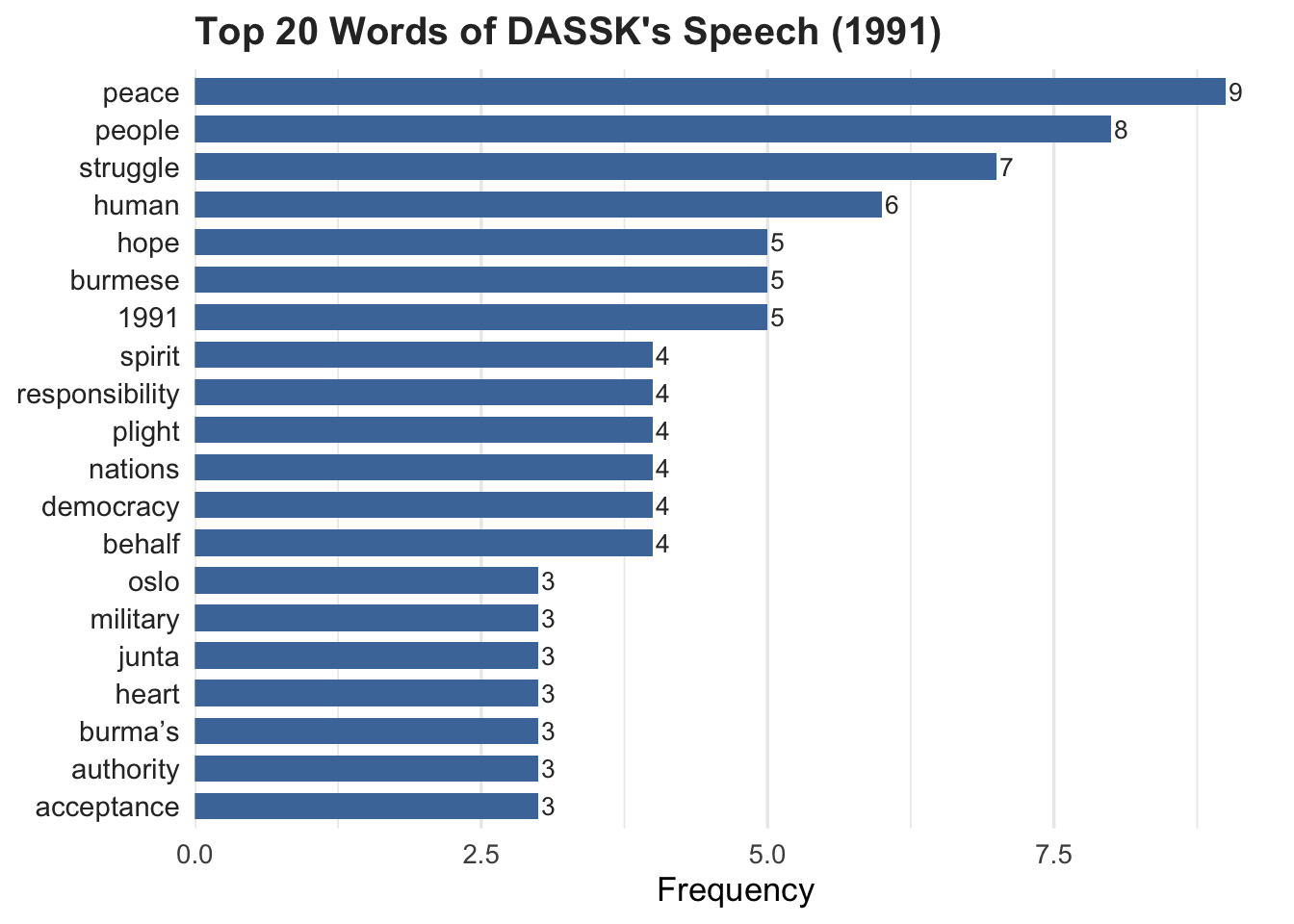

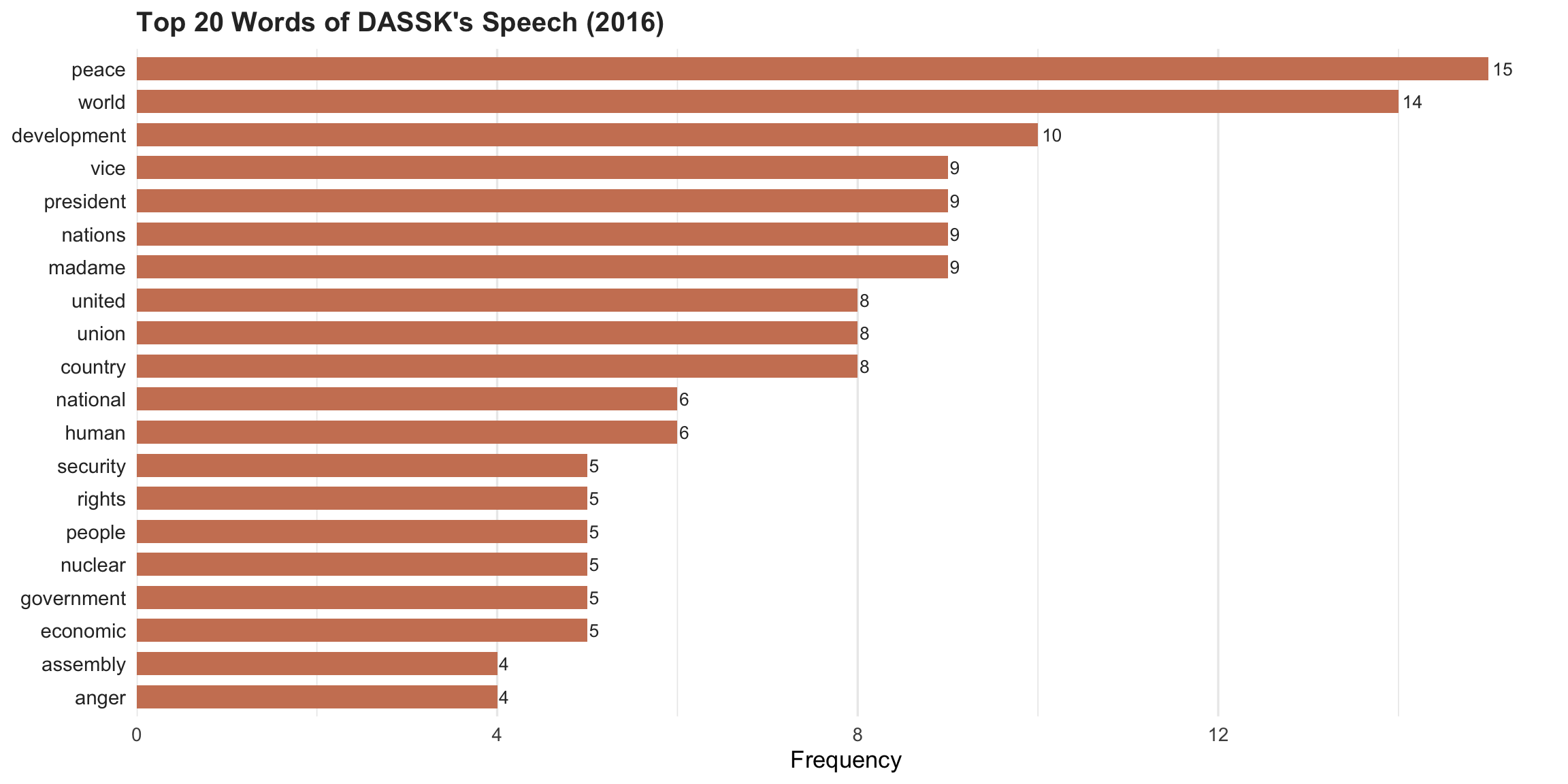
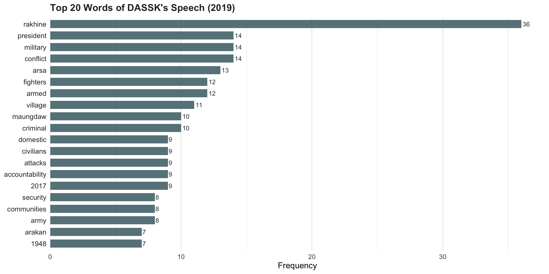
This process is repeated to analyse the other speeches (or could be more).

Word frequencies Comparison

The code combines the cleaned word lists from 1991, 2016, and 2019, tags each word with its year, and calculates how often each word appears as a proportion of that speech’s total words. Using 1991 as the baseline, it compares these proportions with the 2016 and 2019 speeches.

#  Word frequencies Comparison ----
all_speeches <- bind_rows(
  mutate(tidy_speech_91,   speech = "1991"),
  mutate(tidy_speech_2016, speech = "2016"),
  mutate(tidy_speech_2019, speech = "2019")
) 

frequency <- bind_rows(
  mutate(tidy_speech_91,   speech = "1991"),
  mutate(tidy_speech_2016, speech = "2016"),
  mutate(tidy_speech_2019, speech = "2019")
) %>%
  mutate(word = str_extract(word, "[a-z']+")) %>%
  filter(!is.na(word), word != "") %>%
  count(speech, word, name = "n") %>%
  group_by(speech) %>%
  mutate(proportion = n / sum(n)) %>%
  ungroup() %>%
  select(-n) %>%
  pivot_wider(names_from = speech, values_from = proportion, values_fill = 0) %>%
  # pivot ONLY comparison years; keep 1991 as a column
  pivot_longer(
    cols = c(`2016`, `2019`),
    names_to = "speech",
    values_to = "proportion"
  ) %>%
  mutate(baseline_prop = .data[["1991"]])

frequency %>%
  filter(proportion > 0, baseline_prop > 0) %>%  # log-safe
  ggplot(aes(x = proportion, y = baseline_prop,
             color = abs(baseline_prop - proportion))) +
  geom_abline(color = "gray60", lty = 2, linewidth = 0.4) +
  geom_jitter(alpha = 0.35, size = 3.2, width = 0.2, height = 0.2, na.rm = TRUE) +
  geom_text(aes(label = word),
            check_overlap = TRUE, vjust = 1.4, size = 3.4,
            color = "black", alpha = 0.9, na.rm = TRUE) +
  scale_x_log10(labels = percent_format()) +
  scale_y_log10(labels = percent_format()) +
  scale_color_gradient(limits = c(0, 0.001), oob = scales::squish,
                       low = "#2b8cbe", high = "#e34a33",
                       name = "Abs. difference") +
  facet_wrap(~ speech, ncol = 2,
             labeller = labeller(speech = c(`2016` = "2016 speech",
                                            `2019` = "2019 speech"))) +
  theme_minimal(base_size = 13) +
  theme(panel.grid.minor = element_blank(),
        panel.grid.major = element_line(color = "gray85", linewidth = 0.3),
        legend.position = "right") +
  labs(y = "1991 speech (baseline)", x = NULL,
       title = "Word frequency comparison vs 1991 baseline")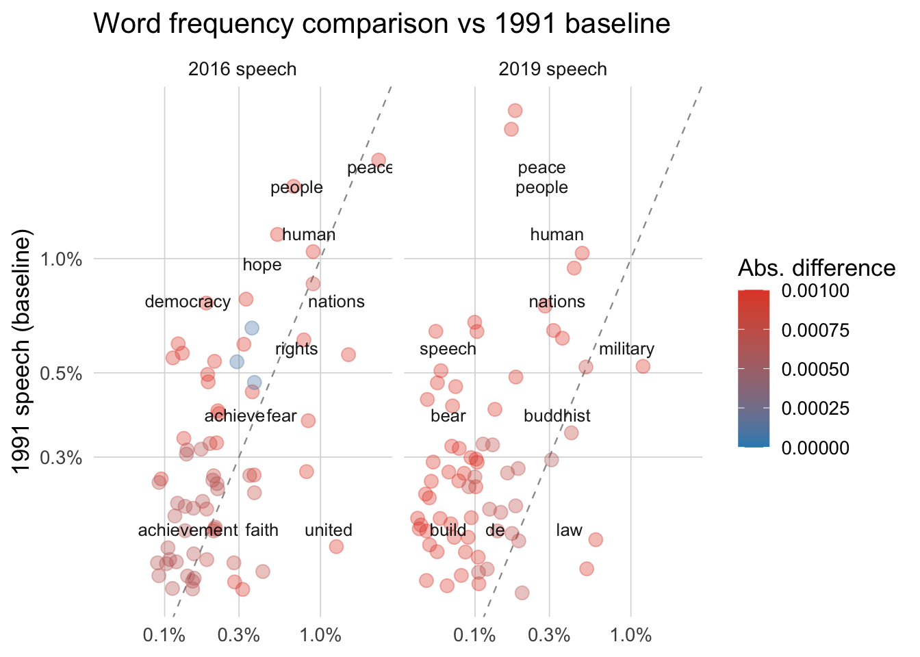

Interpretation of Word Frequencies Comparison

The results are plotted on a log–log scatterplot, where words on the diagonal are used at similar rates in both speeches, and points further away show bigger shifts in emphasis. Colour highlights the size of these changes, and separate panels show the 2016 and 2019 comparisons side by side. The comparison shows that core themes like people, peace, and rights appear in all three speeches but were proportionally more prominent in 1991. The 2016 speech retains much of this earlier focus, while the 2019 speech introduces greater emphasis on context-specific terms such as military, law, and buddhist, reflecting a shift toward governance and legal issues. Overall, the results suggest a move from the moral and humanitarian tone of 1991 toward language shaped by the political and institutional challenges of later years.

The words “Peace” and “Conflict” in speeches

# Only Selected Words ----
all_speeches %>%
  filter(word %in% c("conflict", "peace")) %>% 
  count(speech, word)

# A tibble: 5 × 3
  speech word         n
  <chr>  <chr>    <int>
1 1991   peace        9
2 2016   conflict     2
3 2016   peace       15
4 2019   conflict    14
5 2019   peace        4

all_speeches %>%
  filter(word %in% c("conflict", "peace")) %>% 
  count(speech, word) %>% 
  ggplot(aes(speech, n, fill = word)) +
  geom_col(position = "fill")+
  labs( y = "n", x = "speech",
title = "The changes of the words Peace and Conflict in DASSK speeches")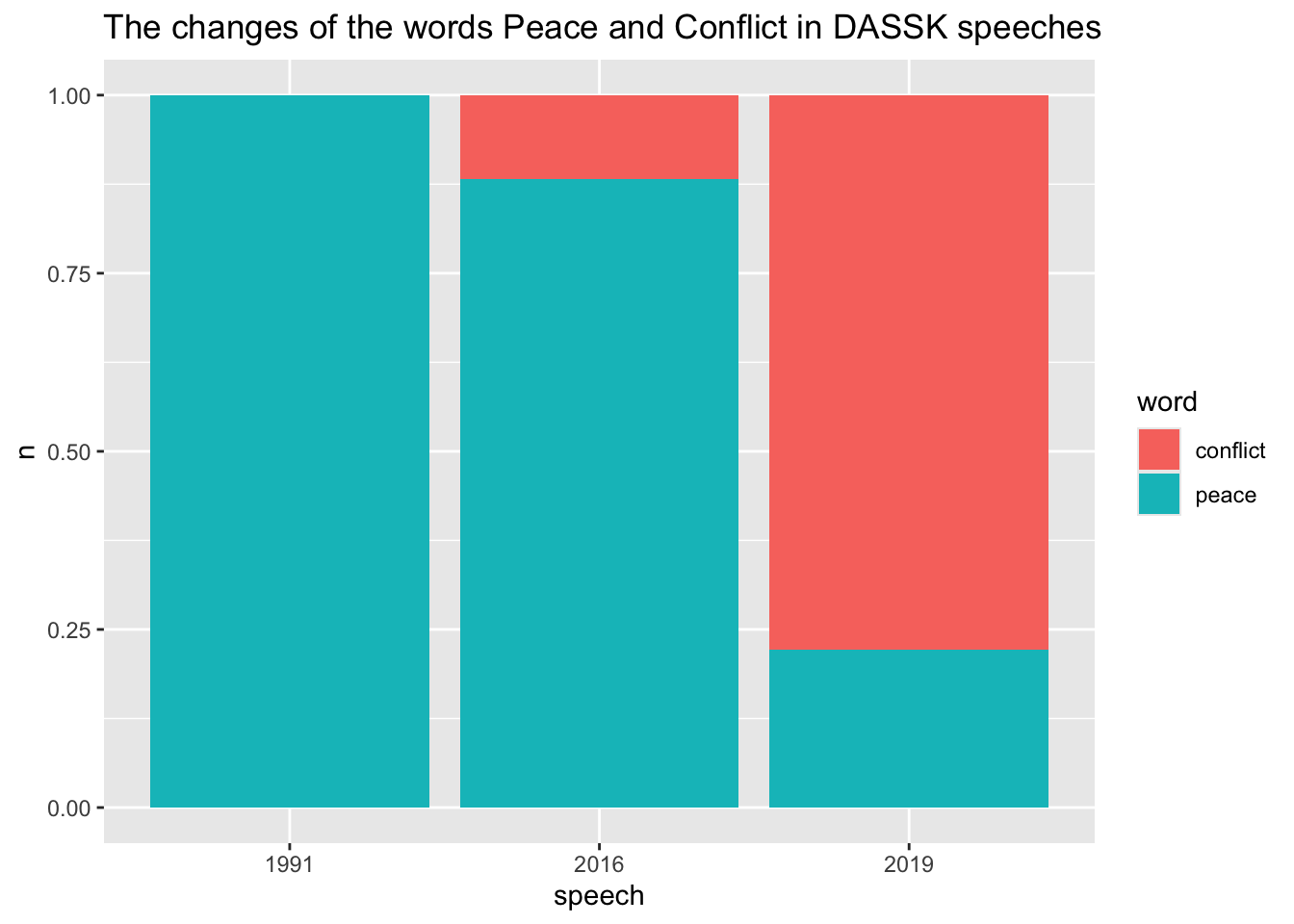

Computing Sentiment Score by AFINN

This code first combines the cleaned, tokenized word lists from the 1991, 2016, and 2019 speeches into a single data frame, adding a speech column to label each year. It then loads the AFINN sentiment lexicon, which assigns each word a score from –5 (strongly negative) to +5 (strongly positive). By joining the speeches with the AFINN lexicon, it keeps only words that have sentiment scores, then calculates, for each speech, the total number of scored tokens, the sum of their sentiment values, and the average sentiment score.

# Combine all speeches into one df
all_speeches <- dplyr::bind_rows(
  dplyr::mutate(tidy_speech_91,   speech = "1991"),
  dplyr::mutate(tidy_speech_2016, speech = "2016"),
  dplyr::mutate(tidy_speech_2019, speech = "2019")
)
stopifnot(exists("all_speeches"), is.data.frame(all_speeches))


# ---- sentiment-afinn ----
afinn <- get_sentiments("afinn")

afinn_scores <- all_speeches %>%
  inner_join(afinn, by = "word") %>%
  group_by(speech) %>%
  summarise(
    tokens_scored = n(),
    sum_score     = sum(value, na.rm = TRUE),
    mean_score    = mean(value, na.rm = TRUE),
    .groups = "drop"
  )

# normalized per 1,000 tokens
speech_sizes <- all_speeches %>% count(speech, name = "n_tokens")

afinn_norm <- afinn_scores %>%
  left_join(speech_sizes, by = "speech") %>%
  mutate(score_per_1k = 1000 * sum_score / n_tokens)

ggplot(afinn_norm, aes(x = reorder(speech, score_per_1k), y = score_per_1k, fill = speech)) +
  geom_col(width = 0.6, show.legend = FALSE) +
  geom_text(aes(label = scales::number(score_per_1k, accuracy = 0.1)),
            vjust = -0.5, size = 4, color = "#333333") +
  scale_fill_manual(values = c("#4575b4", "#91bfdb", "#d73027")) +
  scale_y_continuous(expand = expansion(mult = c(0, 0.1))) +
  labs(
    title = "AFINN Sentiment — Normalized by Speech Length",
    subtitle = "Score per 1,000 tokens",
    x = NULL, y = "Sentiment score / 1,000 words"
  ) +
  theme_minimal(base_size = 14)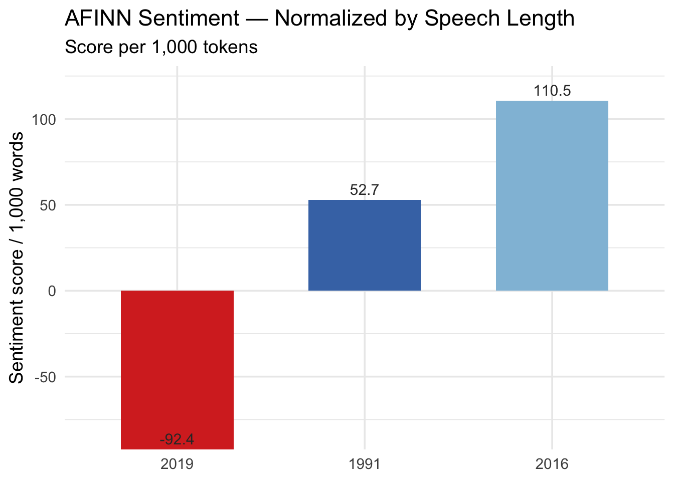

Because the speeches differ in length, the total sentiment scores are normalized by dividing by the number of words in each speech and multiplying by 1,000, giving a “score per 1,000 words” measure.

Interpretation of AFINN Sentiment

When Daw Aung San Suu Kyi became the State Counsellor of then government in 2016, the speech made to the General Debate of UN General Assembly registers the highest positive sentiment at 110.5, indicating a notably optimistic or affirmative tone compared with the other two speeches. The 1991 Nobel Award acceptance speech also carries a positive tone, though at a lower level of 52.7, suggesting a more balanced or measured emotional profile. In contrast, when Daw Aung San Suu Kyi deliver the speech as agent of then Myanmar government at the International Court of Justice, The Hague, the speech stands out with a strongly negative score of –92.4, reflecting a shift toward language containing more negative or critical expressions. This pattern suggests an evolution from the moral optimism of 1991 to the high positivity of 2016, followed by a marked downturn in emotional tone in 2019, likely influenced by the political and diplomatic pressures surrounding that later address.

Discussion

The findings point to a clear rhetorical shift in Daw Aung San Suu Kyi’s leadership, from moral advocacy and activist leadership toward pragmatic statecraft. In 1991, her moderately positive tone embodied the universalist ideals of a moral opposition figure, grounded in human rights and democratic principles. By 2016, the heightened positivity reflected an agenda-setting phase aimed at consolidating political legitimacy and advancing reform within the constraints of partial civilian rule. The sharp turn to negativity in 2019 signaled a defensive, sovereignty-focused discourse shaped by the political imperatives of regime survival amid mounting international criticism. This progression illustrates how leadership rhetoric evolves as political roles transition from principled opposition to the strategic calculations required in governance.

Limitation and Future Research

A key limitation of this study is its reliance on a small set of speeches delivered to international audiences, which may not fully capture the range of Daw Aung San Suu Kyi’s rhetorical strategies across different contexts. The analysis also depends on dictionary-based sentiment tools, which can overlook nuance and culturally specific expressions. Future research could broaden the dataset to include domestic speeches, interviews, and policy statements, apply more advanced natural language processing techniques, and undertake comparative analysis with other Southeast Asian leaders who have navigated both activist and statesman roles, to deepen understanding of regional patterns in political communication.

References:

Aung San Suu Kyi – Acceptance Speech. NobelPrize.org. Nobel Prize Outreach 2025. Tue. 12 Aug 2025. https://www.nobelprize.org/prizes/peace/1991/kyi/acceptance-speech/

Silge, Julia, David Robinson, and David Robinson. Text mining with R: A tidy approach. Boston (MA): O’reilly, 2017.

United Nations. “Myanmar - Minister for Foreign Affairs Addresses General Debate, 71st Session.” UN Web TV, United Nations, video, 21 September 2016, https://webtv.un.org/en/asset/k12/k12rs94q5t. Accessed 12 Aug. 2025.

United Nations. “ICJ/Aung San Suu Kyi” UN Web TV, United Nations, video, 11 December 2019, https://media.un.org/unifeed/en/asset/d251/d2513117. Accessed 12 Aug. 2025.

sessionInfo()

Save RAM space into Hard disk

save.image("Our_First_RMarkdown.RData")